GIS
- QGIS
- GRASS
- SAGA
- ArcGIS
![]()
sf: simple features is an open standard endorsed by the Open Geospatial Consortium.
library(tidyverse)
library(sf)
system.file("gpkg/nc.gpkg", package="sf") |>
    read_sf() -> nc
nc.32119 <- st_transform(nc, 'EPSG:32119')
nc.32119 |>
    select(BIR74) |>
    plot(graticule = TRUE, axes = TRUE)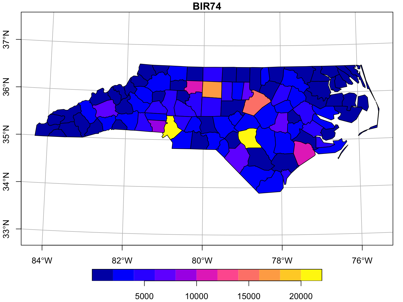
BIR74 is birth counts over the region (North Carolina)
| type | description |
|---|---|
POINT |
single point geometry |
MULTIPOINT |
set of points |
LINESTRING |
single linestring (two or more points connected by straight lines) |
MULTILINESTRING |
set of linestrings |
POLYGON |
exterior ring with zero or more inner rings, denoting holes |
MULTIPOLYGON |
set of polygons |
GEOMETRYCOLLECTION |
set of the geometries above |
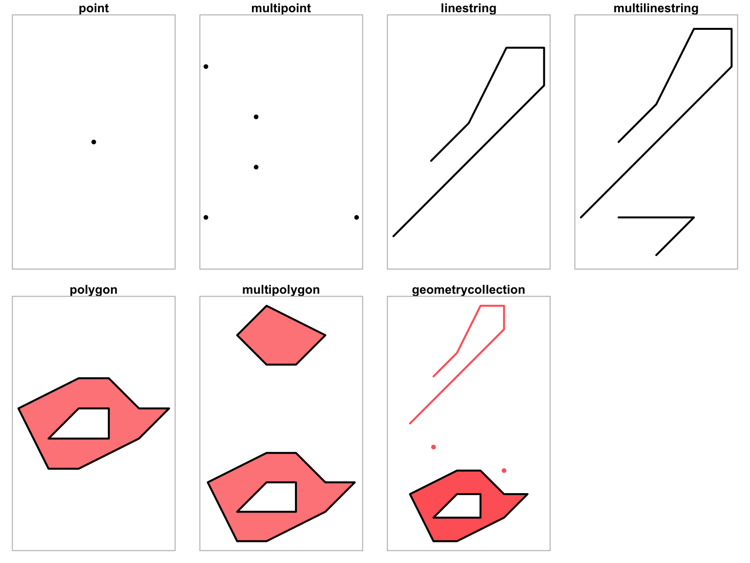
Other geometries include: CIRCULARSTRING, COMPOUNDCURVE, CURVEPOLYGON, MULTICURVE, MULTISURFACE, CURVE, SURFACE, TIN, TRIANGLE.
Source: Pebesma, 2022 (Chapter 3)
sffilter
Select all counties less than 50 km away from Orange county:
orange <- nc |> dplyr::filter(NAME == "Orange")
wd <- st_is_within_distance(
    nc, orange,
    units::set_units(50, km))

o50 <- nc |> dplyr::filter(lengths(wd) > 0)
nrow(o50)
[1] 17Remember: The experession
::means accessing an object from a namespace (e.g. a function from a package)
og <- st_geometry(orange)
plot(st_geometry(o50), lwd = 2)
plot(og, col = 'orange', add = TRUE)
plot(st_buffer(og, units::set_units(50, km)), add = TRUE, col = NA, border = 'brown')
plot(st_geometry(nc), add = TRUE, border = 'grey')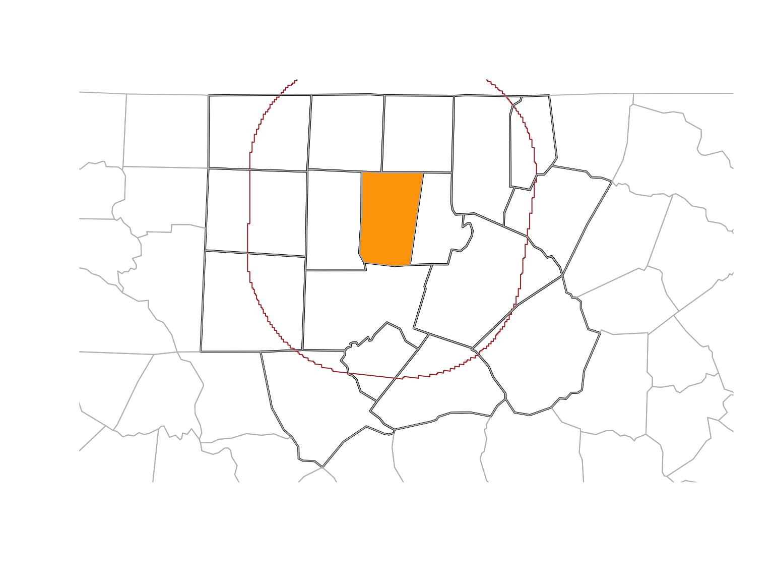
Work on spatial predicates instead of common columns. One needs to define spatially matching records
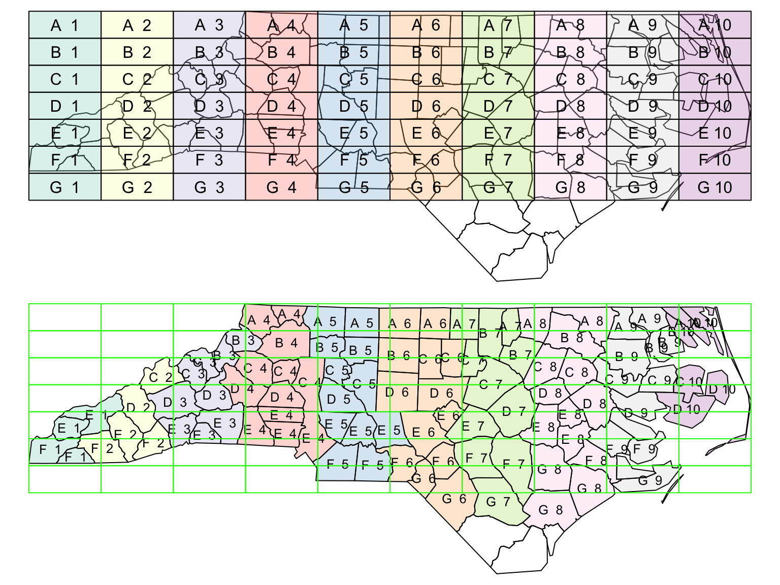
gr <- st_sf(
    label = apply(
        expand.grid(1:10, LETTERS[10:1])[,2:1], 1,
        paste0, collapse = " "),
    geom = st_make_grid(nc))

gr$col <- sf.colors(10, categorical = TRUE, alpha = .3)

# cut, to verify that NA's work out:
gr <- gr[-(1:30),]

# spatial join
suppressWarnings(nc_j <- st_join(nc, gr, largest = TRUE))

# graphics
par(mfrow = c(2,1), mar = rep(0,4))
plot(st_geometry(nc_j))
plot(st_geometry(gr), add = TRUE, col = gr$col)
text(st_coordinates(st_centroid(st_geometry(gr))), labels = gr$label)
# the joined dataset:
plot(st_geometry(nc_j), border = 'black', col = nc_j$col)
text(st_coordinates(st_centroid(st_geometry(nc_j))), labels = nc_j$label, cex = .8)
plot(st_geometry(gr), border = 'green', add = TRUE)
Example of largest = TRUE
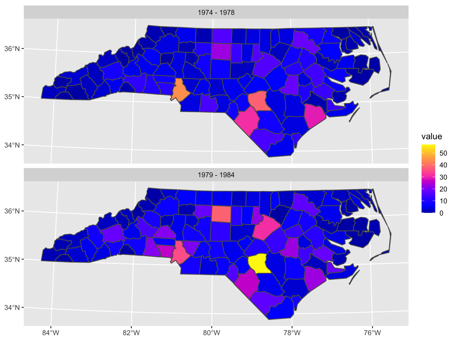
year_labels <- c(
    "SID74" = "1974 - 1978", "SID79" = "1979 - 1984")

nc_longer <- nc.32119 |>
    select(SID74, SID79) |>
    pivot_longer(starts_with("SID"))

## Ggplot friendly but needs long format
## objects to work with facets:

ggplot() +
    # geom_sf undestands special features!
    geom_sf(data = nc_longer, aes(fill = value)) +
    facet_wrap(~ name, ncol = 1,
               labeller = labeller(name = year_labels)) +
    scale_y_continuous(breaks = 34:36) +
    scale_fill_gradientn(colors = sf.colors(20)) +
    theme(panel.grid.major = element_line(color = "white"))