Networks

Martin Grandjean, CC BY-SA 4.0, via Wikimedia Commons

Quiz

What are the basic data structures in R?

Objects & Classes

Object classess depending on dimensions and type
Dimensions	Homogeneous	Heterogeneous
1	Vector	List
2	Matrix	Data Frame
3	Array	NA

Networks are matrices

Adjacency matrix (squared)
- Symmetric = Undirected
- Asymmetric = Directed
Incidence matrix (rectangular)
- Bipartite / hypergraphs
Edgelist
Jargon check
- Node = vertex
- Link = edge = arc
- Network = graph

Networks in R

statnet::network

Social sciences and statistics
Strong support for statistical modelling
Network size = small - medium

`statnet`

Create a network

library(network)
mat <- matrix(rbinom(25,1,0.3), 5,5)
diag(mat) <- 0
net <- network(mat)
summary(net)

## Network attributes:
##   vertices = 5
##   directed = TRUE
##   hyper = FALSE
##   loops = FALSE
##   multiple = FALSE
##   bipartite = FALSE
##  total edges = 5 
##    missing edges = 0 
##    non-missing edges = 5 
##  density = 0.25 
## 
## Vertex attributes:
##   vertex.names:
##    character valued attribute
##    5 valid vertex names
## 
## No edge attributes
## 
## Network adjacency matrix:
##   1 2 3 4 5
## 1 0 0 0 0 0
## 2 1 0 0 0 1
## 3 0 0 0 0 1
## 4 0 0 0 0 0
## 5 0 0 1 1 0

`statnet`

Adjacency matrix are used in bipartite graphs

library(network)
mat <- matrix(rbinom(30,1,0.3), 6,5)
diag(mat) <- 0
net <- network(mat)
summary(net)

## Network attributes:
##   vertices = 11
##   directed = FALSE
##   hyper = FALSE
##   loops = FALSE
##   multiple = FALSE
##   bipartite = 6
##  total edges = 10 
##    missing edges = 0 
##    non-missing edges = 10 
##  density = 0.1818182 
## 
## Vertex attributes:
##   vertex.names:
##    character valued attribute
##    11 valid vertex names
## 
## No edge attributes
## 
## Network adjacency matrix:
##   7 8 9 10 11
## 1 0 0 0  0  0
## 2 1 0 0  1  1
## 3 1 0 0  0  0
## 4 1 1 0  0  0
## 5 1 0 1  0  0
## 6 1 0 1  0  0

Edgelists allow for more compact formats

library(tidyverse)
dat <- tribble(
    ~from, ~to, ~value,
    "Agnes", "Mary", 4,
    "John", "Andrea", 2,
    "Mary", "John", 1,
    "Ingo", "Mary", 6,
    "Stefan", "Ingo", 1
)
net <- network(dat)
summary(net)

## Network attributes:
##   vertices = 6
##   directed = TRUE
##   hyper = FALSE
##   loops = FALSE
##   multiple = FALSE
##   bipartite = FALSE
##  total edges = 5 
##    missing edges = 0 
##    non-missing edges = 5 
##  density = 0.1666667 
## 
## Vertex attributes:
##   vertex.names:
##    character valued attribute
##    6 valid vertex names
## 
## Edge attributes:
## 
##  value:
##    numeric valued attribute
##    attribute summary:
##    Min. 1st Qu.  Median    Mean 3rd Qu.    Max. 
##     1.0     1.0     2.0     2.8     4.0     6.0 
## 
## Network adjacency matrix:
##        Agnes John Mary Ingo Stefan Andrea
## Agnes      0    0    1    0      0      0
## John       0    0    0    0      0      1
## Mary       0    1    0    0      0      0
## Ingo       0    0    1    0      0      0
## Stefan     0    0    0    1      0      0
## Andrea     0    0    0    0      0      0

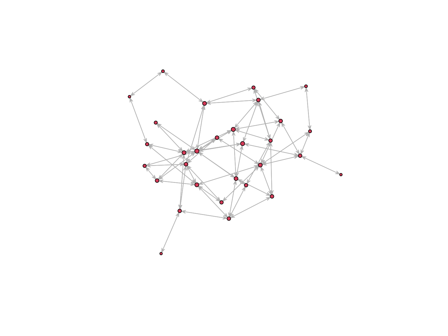
Network statistics

Who is more central?

sna: social network analysis

library(sna) 
net <- network(
    rgraph(n = 30, tprob = 0.15, mode = "graph")) #digraph for directed
# number of connections
degree(net)

##  [1]  4 10 10  8  6  2  4  4  6  6 10 12  2 14  8  6  8  8  6  6 12 18 12 10 10
## [26] 12 10  6 10  4

On a directed network you will have in- and out- degree.

Butts, T. 2008. Social Network Analysis with sna. Journal of Statistical Software

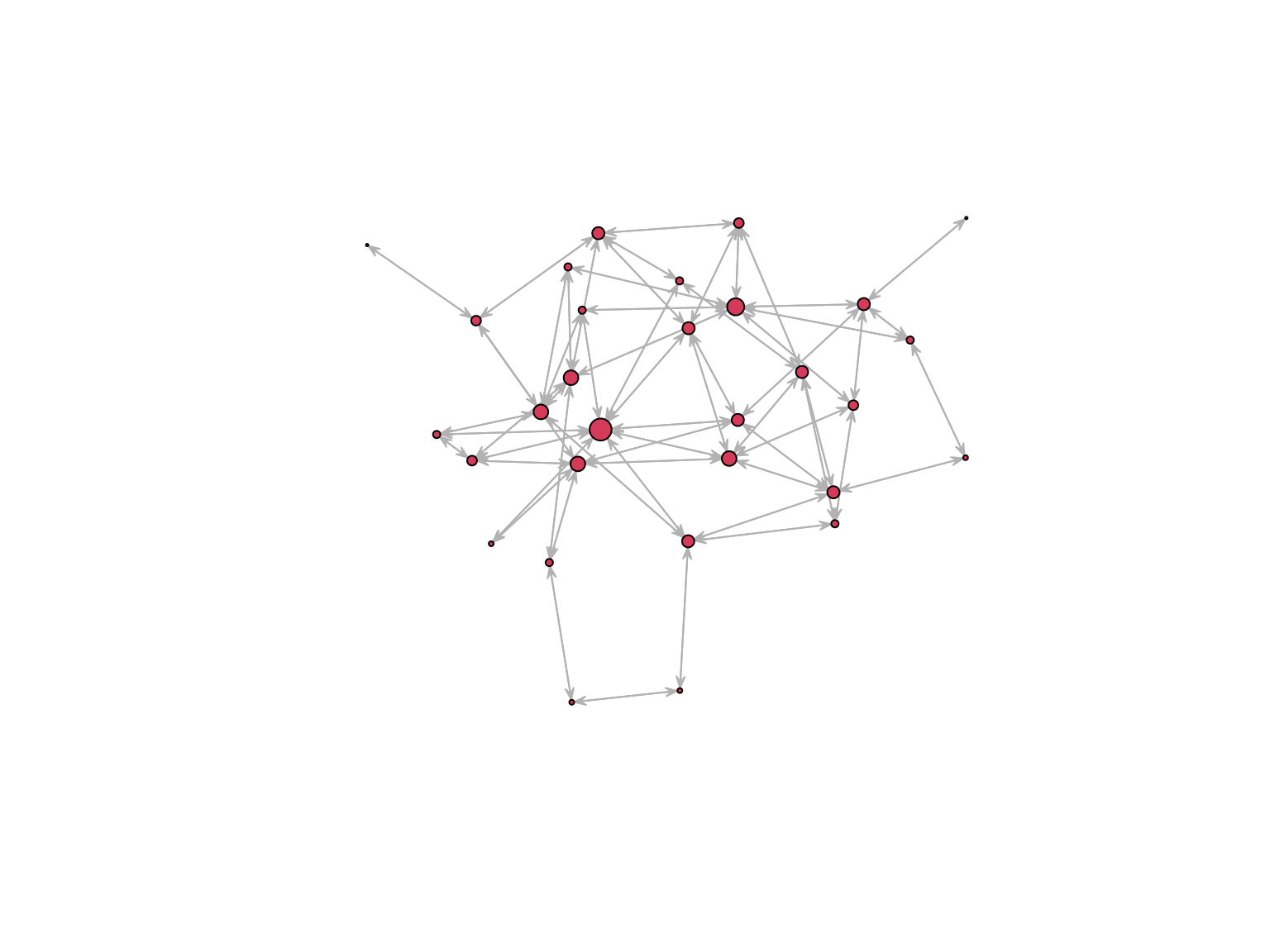
Network statistics

Betweenness measures the extent to which a vertex lie in the paths between other vertices

plot.network(
    net, edge.col = "grey75", edge.lwd = 0.05,
    vertex.cex =  betweenness(net, gmode = "graph")/10)

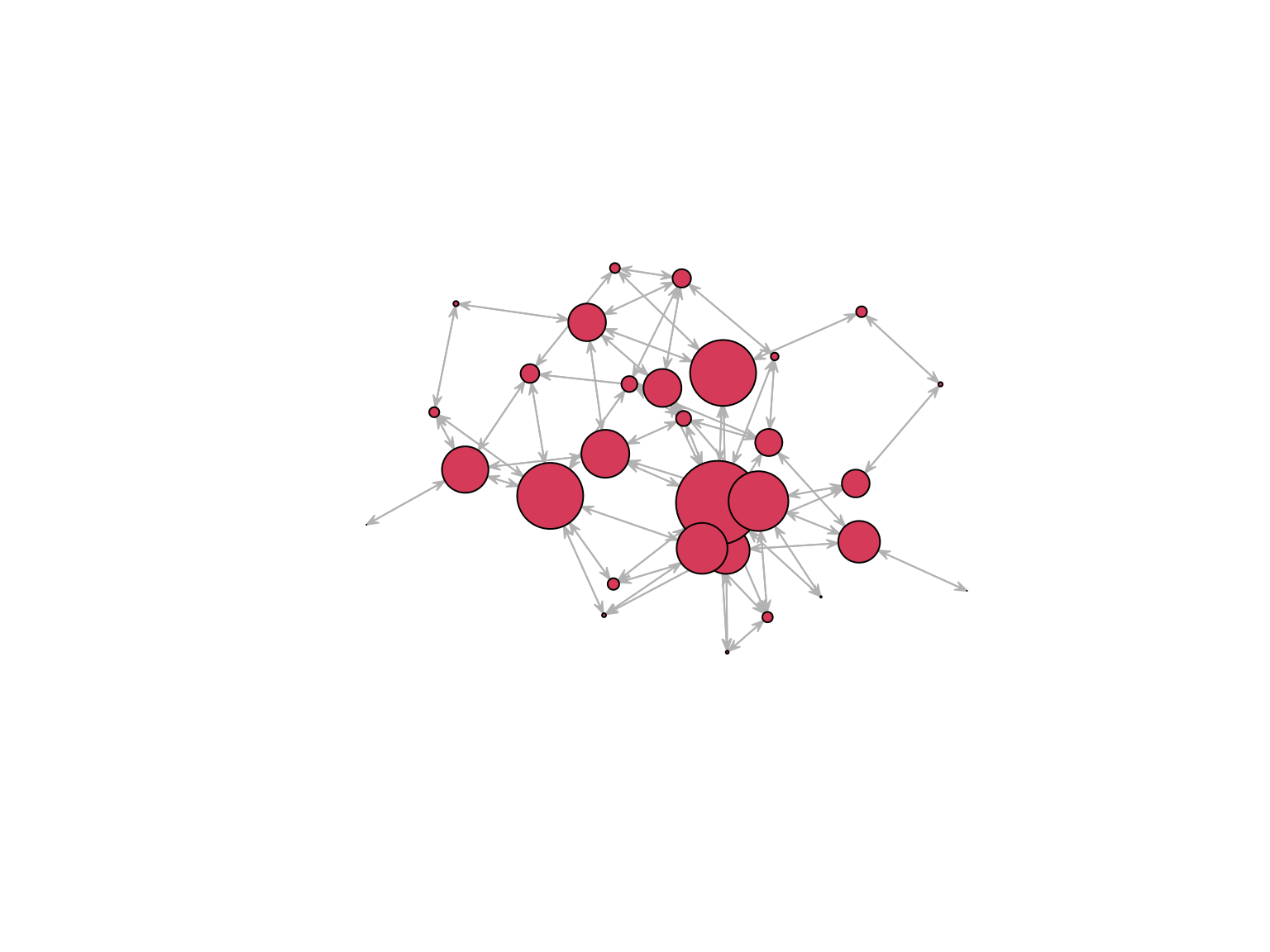On a directed network direction is accounted for.

Butts, T. 2008. Social Network Analysis with sna. Journal of Statistical Software

Centrality

Degree
Betweenness
Closeness
Eigenvector
PageRank
Katz
Hubs
Bonacich Power
Cliques and cores

Example

Rocha et al. 2015. PlosOne

One mode vs bipartite

Most network operations are simply linear algebra on matrices

Useful math to study co-authorship networks, people and groups (e.g. company boards, investors), affiliation, co-occurrence, pollination, gene-disease, drug discovery, among many others

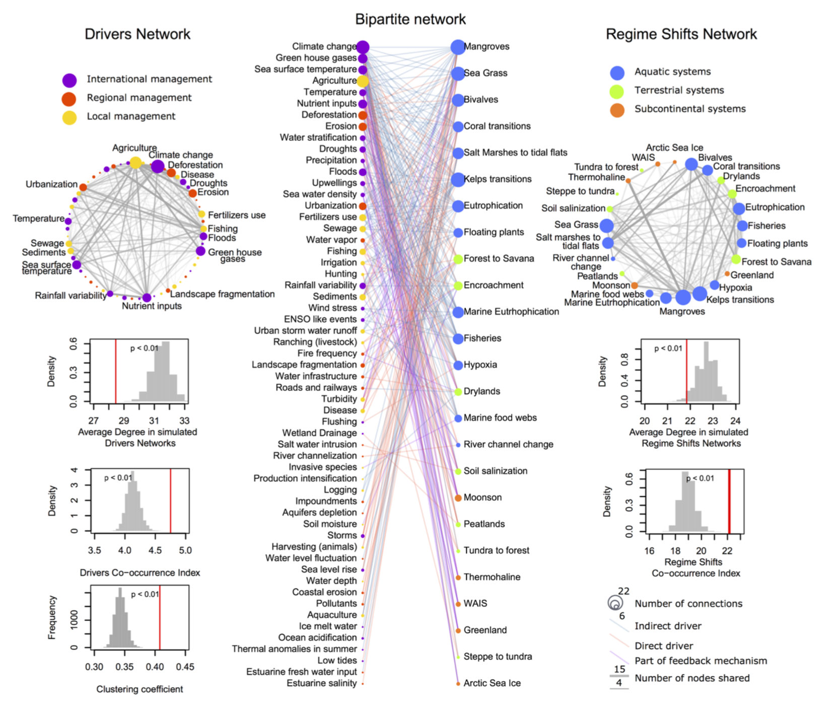
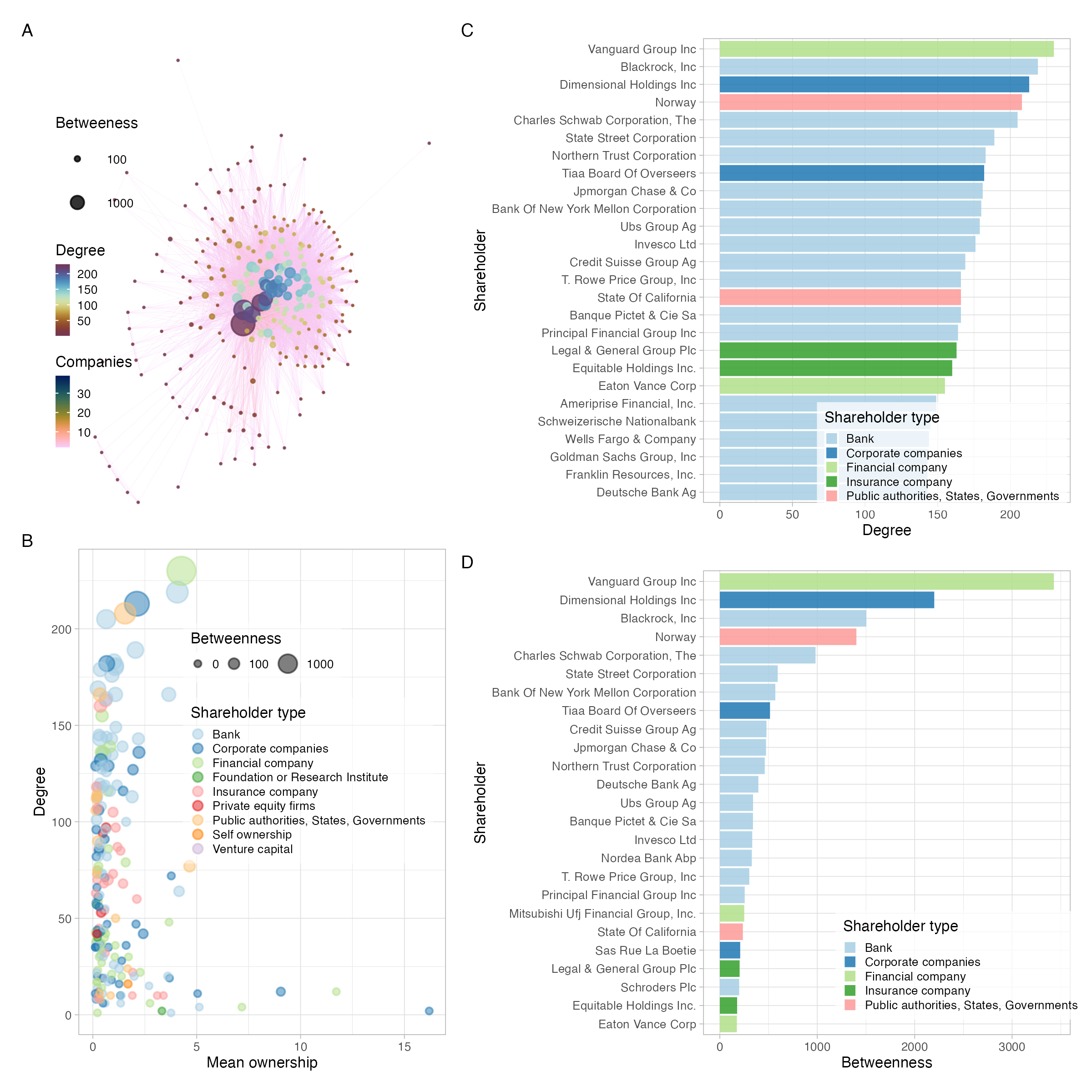
Who has the agency to make a difference?

Galaz et al 2022 Beijer Discussion Papers

Another example: path analysis

Rocha, J, et al . Cascading regime shifts within and across scales. Science 362, 1379–1383 (2018)

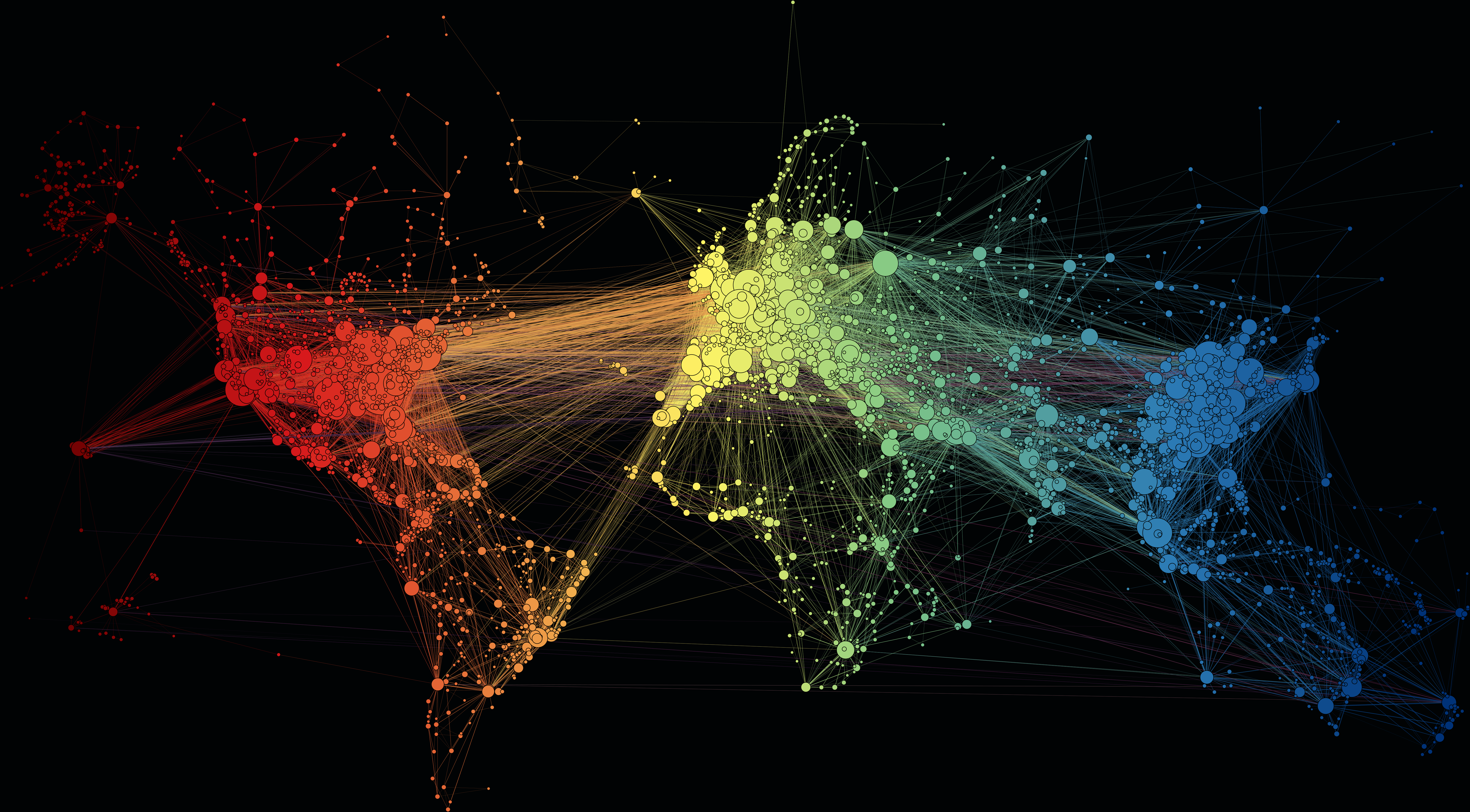
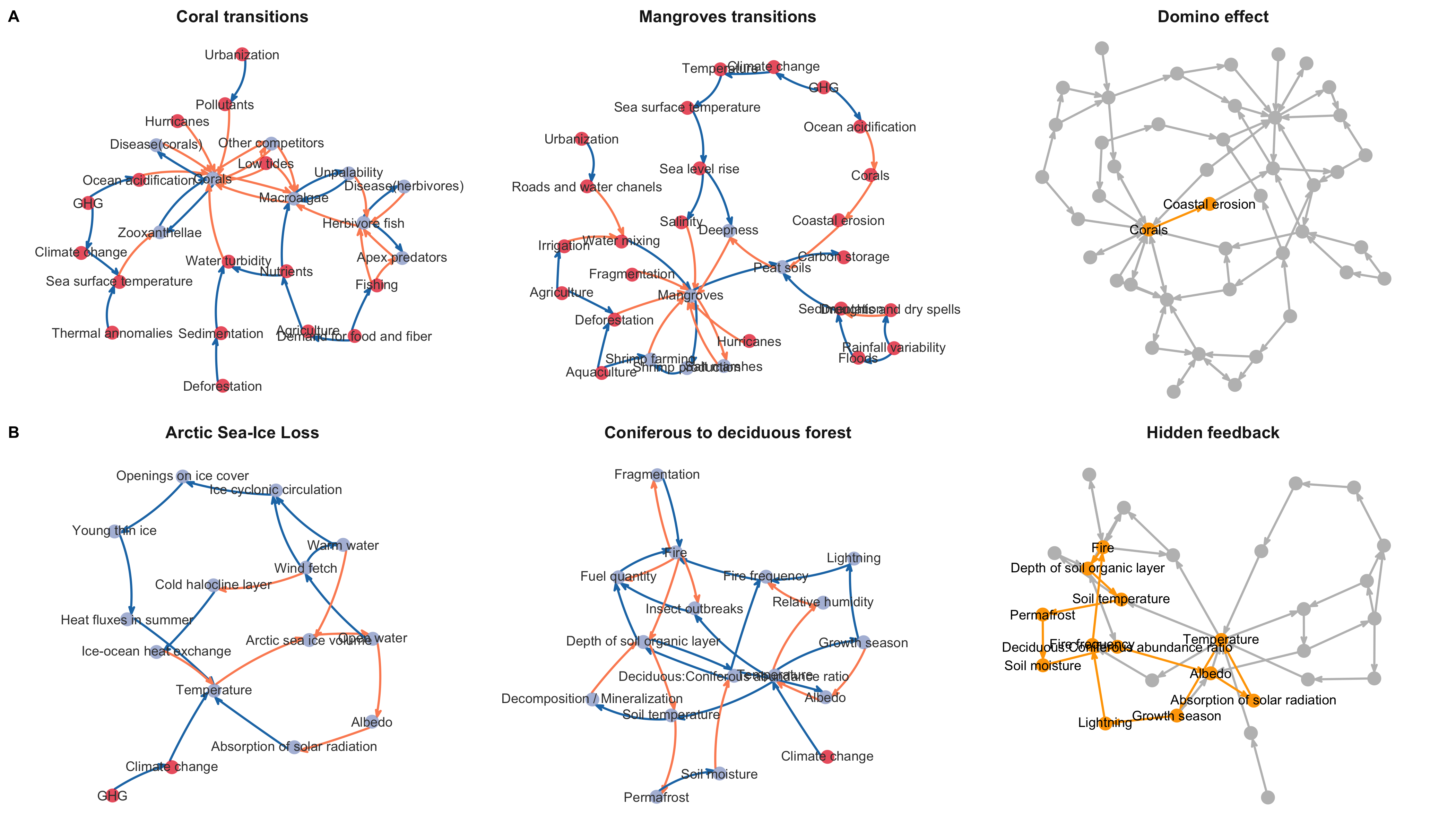
A worked example

example

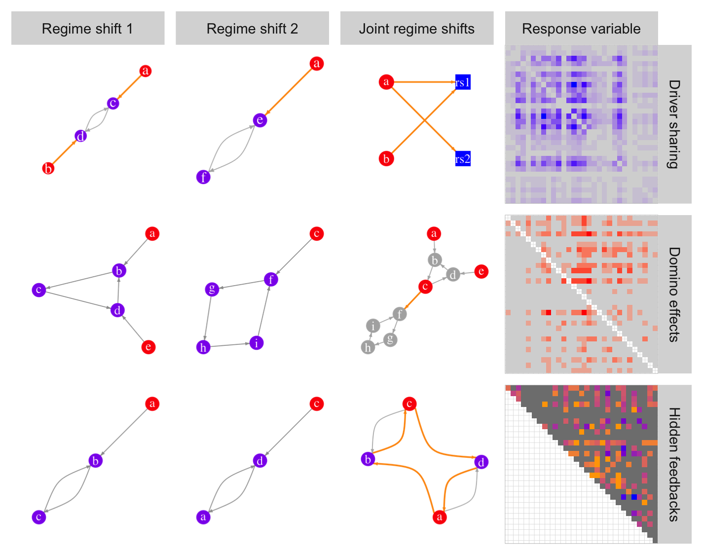
Cascading effects

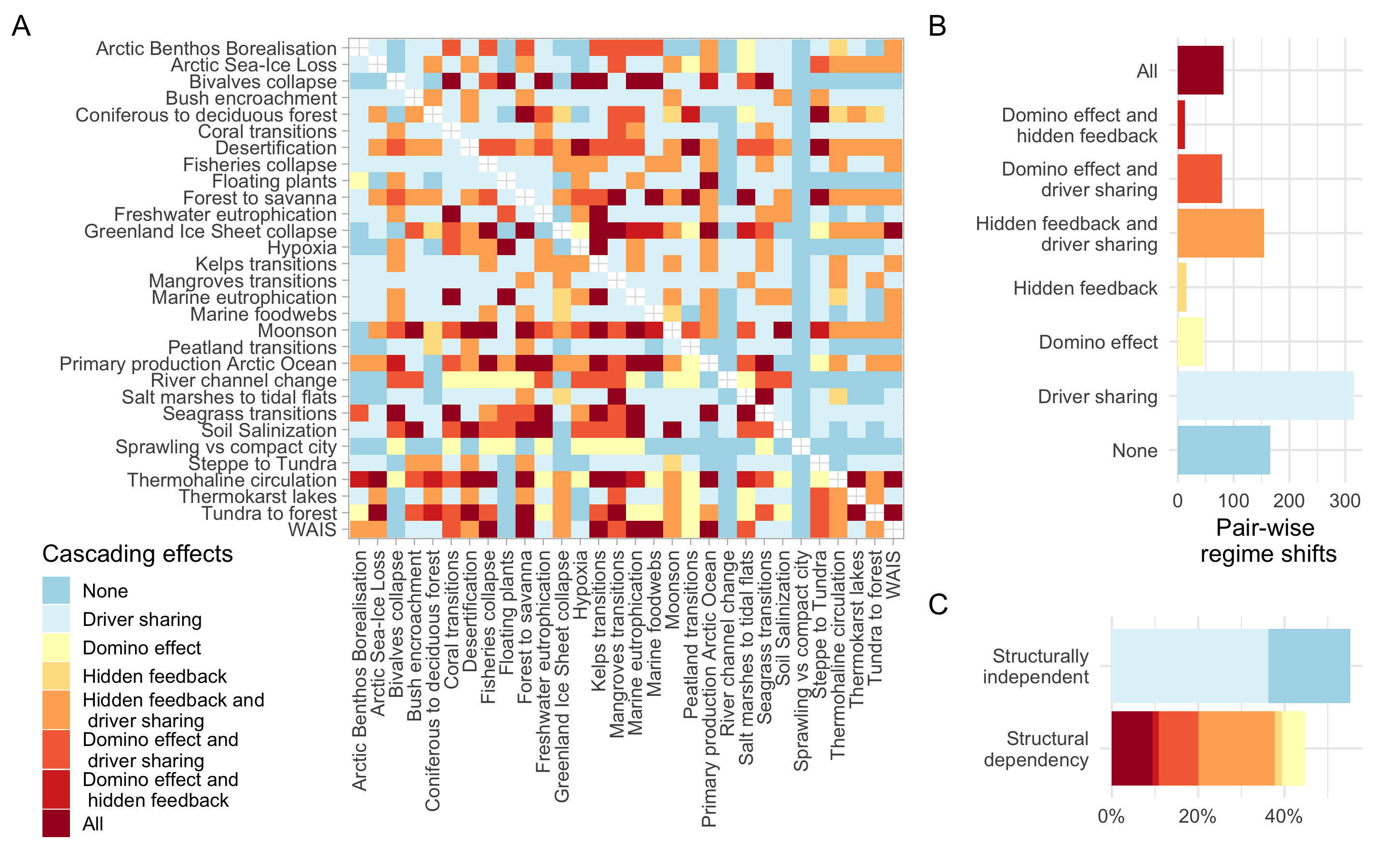
~45% of the regime shift couplings analyzed present structural dependencies in the form of one-way interactions for the domino effect or two-way interactions for hidden feedbacks

Rocha, J. et al 2018. Science

`igraph`

Strong focus on algorithms
Optimized to handle large objects
Slightly different syntax

Be aware of conflicts between packages

detach(package:sna)
detach(package:network)
library(igraph)

## 
## Attaching package: 'igraph'

## The following objects are masked from 'package:lubridate':
## 
##     %--%, union

## The following objects are masked from 'package:dplyr':
## 
##     as_data_frame, groups, union

## The following objects are masked from 'package:purrr':
## 
##     compose, simplify

## The following object is masked from 'package:tidyr':
## 
##     crossing

## The following object is masked from 'package:tibble':
## 
##     as_data_frame

## The following objects are masked from 'package:stats':
## 
##     decompose, spectrum

## The following object is masked from 'package:base':
## 
##     union

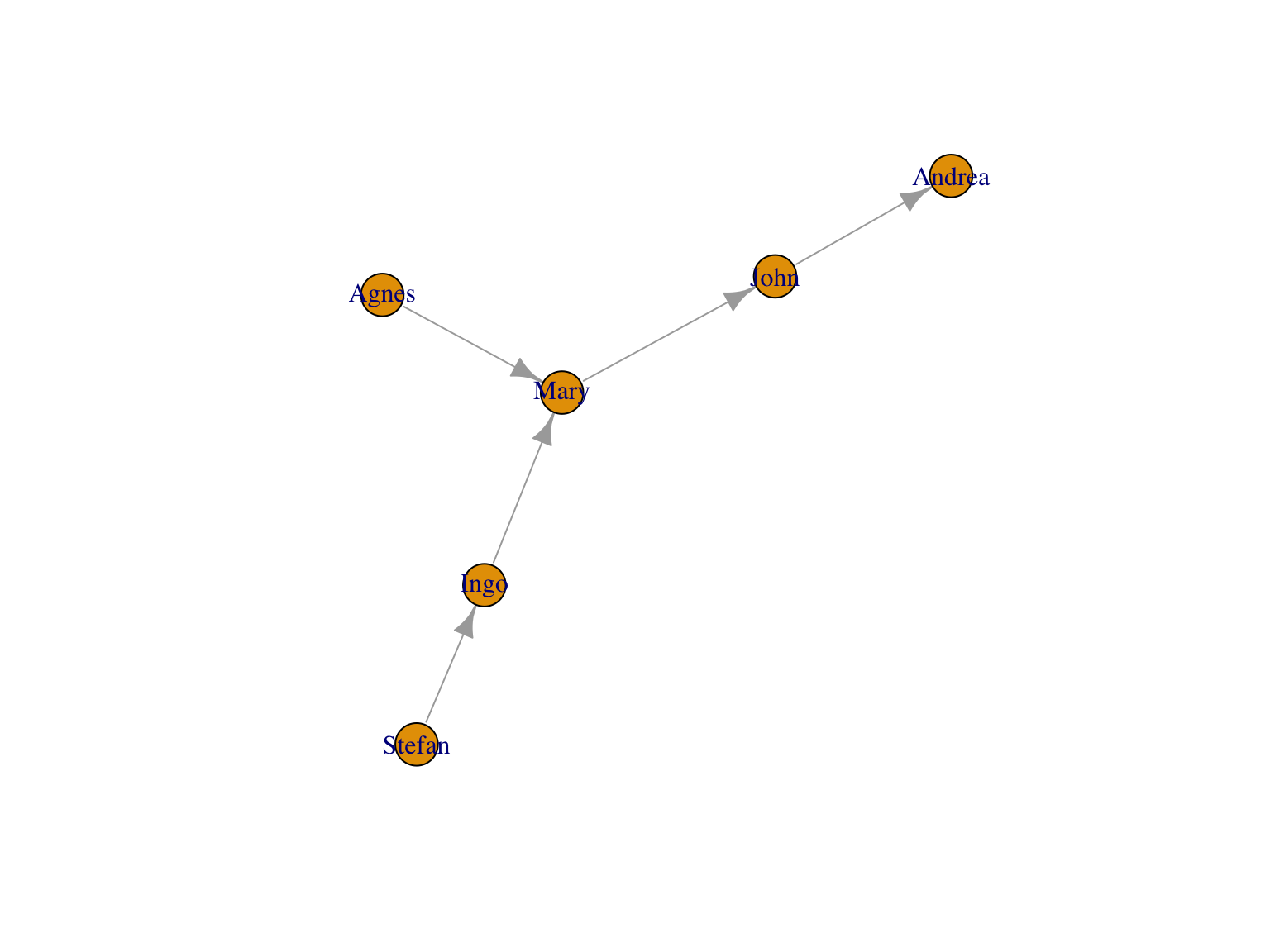
`igraph`

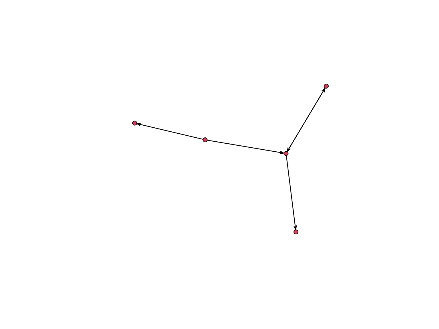
Create a graph

g <- graph_from_edgelist(
    as.matrix(dat[,1:2]))
g

## IGRAPH 578bfae DN-- 6 5 -- 
## + attr: name (v/c)
## + edges from 578bfae (vertex names):
## [1] Agnes ->Mary   John  ->Andrea Mary  ->John   Ingo  ->Mary   Stefan->Ingo

Other options

make_tree(10, 2)
graph_from_dataframe()
graph_from_incidence_matrix()
graph_from_adjancecy_matrix()

Complex objects

Networks are complex objects:

Matrix or edgelist
Node attributes
Edge attributes

Useful for visualization and statistical modelling

Motifs

igraph::triad_census(g)

##  [1]  5 10  0  0  1  4  0  0  0  0  0  0  0  0  0  0

Vertex attributes

statnet

net %v% "sex" <- sample(c(0,1), 30, replace = TRUE)
set.vertex.attribute(net, "sex", value = sample(c(0,1), 30, replace = TRUE))
get.vertex.attribute(net, "sex")

igraph

V(g)

## + 6/6 vertices, named, from 578bfae:
## [1] Agnes  Mary   John   Andrea Ingo   Stefan

V(g)$sex <- c("F", "F", "M", "F", "M", "M")
vertex_attr(g)

## $name
## [1] "Agnes"  "Mary"   "John"   "Andrea" "Ingo"   "Stefan"
## 
## $sex
## [1] "F" "F" "M" "F" "M" "M"

Edge attributes

statnet

net %e% "type" <- "co-workers"
set.vertex.attribute(net, "sex", value = sample(c(0,1), 30, replace = TRUE))
get.vertex.attribute(net, "sex")

igraph

E(g)

## + 5/5 edges from 578bfae (vertex names):
## [1] Agnes ->Mary   John  ->Andrea Mary  ->John   Ingo  ->Mary   Stefan->Ingo

E(g)$sport <- c("chess", "swimming", "swimming", "climbing", "fencing")
edge_attr(g)

## $sport
## [1] "chess"    "swimming" "swimming" "climbing" "fencing"

E(g)$sport

## [1] "chess"    "swimming" "swimming" "climbing" "fencing"

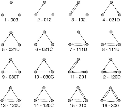
Network modelling

Mechanisms for network formation

Random (Erdos-Renyi)
Small-world (Watts-Strogatz)
Preferential attachment (Barabasi-Albert)
Homophily vs influence
Assortativity
Motifs mixture

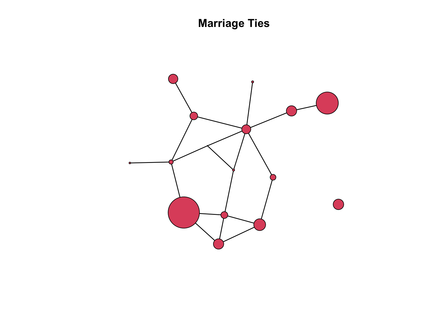
Network modelling

detach(package:igraph)
library(ergm)
data(flo)
flomarriage <- network(flo,directed=FALSE)
flomarriage %v% "wealth" <- c(10,36,27,146,55,44,20,8,42,103,48,49,10,48,32,3)
fit1 <- ergm(flomarriage ~ edges + absdiff("wealth"))
summary(fit1)

## Call:
## ergm(formula = flomarriage ~ edges + absdiff("wealth"))
## 
## Maximum Likelihood Results:
## 
##                 Estimate Std. Error MCMC % z value Pr(>|z|)    
## edges          -1.457666   0.354532      0  -4.112   <1e-04 ***
## absdiff.wealth -0.004176   0.007387      0  -0.565    0.572    
## ---
## Signif. codes:  0 '***' 0.001 '**' 0.01 '*' 0.05 '.' 0.1 ' ' 1
## 
##      Null Deviance: 166.4  on 120  degrees of freedom
##  Residual Deviance: 107.8  on 118  degrees of freedom
##  
## AIC: 111.8  BIC: 117.4  (Smaller is better. MC Std. Err. = 0)

Network modelling

fit2 <- ergm(flomarriage ~ edges + absdiff("wealth") + triangle)
summary(fit2)

## Call:
## ergm(formula = flomarriage ~ edges + absdiff("wealth") + triangle)
## 
## Monte Carlo Maximum Likelihood Results:
## 
##                 Estimate Std. Error MCMC % z value Pr(>|z|)   
## edges          -1.467774   0.503880      0  -2.913  0.00358 **
## absdiff.wealth -0.004324   0.007631      0  -0.567  0.57095   
## triangle        0.072487   0.602304      0   0.120  0.90421   
## ---
## Signif. codes:  0 '***' 0.001 '**' 0.01 '*' 0.05 '.' 0.1 ' ' 1
## 
##      Null Deviance: 166.4  on 120  degrees of freedom
##  Residual Deviance: 107.8  on 117  degrees of freedom
##  
## AIC: 113.8  BIC: 122.1  (Smaller is better. MC Std. Err. = 0.00496)

Visualization

plot() commands from each package
networkD3 wraps a nice java script library (interactive)
ggnetwork & ggraph uses ggplot syntax
graph package (circular plots)
circlos package for chord diagrams (interactive)

Play around with your own!

Resources

Online tutorials (often offered in Sunbelt, NetSci)
- Katya Ognyanova: https://kateto.net/tutorials/
Books:
- Introduction to Networks by Mark Newman (2010)

Exercise

Data

Study the academic production of SRC!

Download the Scopus record of all SRC publications by 2022

Link: https://stockholmuniversity.box.com/s/35ydfdtm8gheh1s1jsrfscj6tj9ixhog

Note: ~25MB csv file

Data

pubs <- read_csv("/Users/juanrocha/Box Sync/Share&Delete/scopus-SRC_221102.csv")

## Rows: 1870 Columns: 20
## ── Column specification ────────────────────────────────────────────────────────
## Delimiter: ","
## chr (17): Authors, Author(s) ID, Title, Source title, Volume, Issue, Art. No...
## dbl  (3): Year, Page count, Cited by
## 
## ℹ Use `spec()` to retrieve the full column specification for this data.
## ℹ Specify the column types or set `show_col_types = FALSE` to quiet this message.

pubs

## # A tibble: 1,870 × 20
##    Authors     `Author(s) ID` Title  Year `Source title` Volume Issue `Art. No.`
##    <chr>       <chr>          <chr> <dbl> <chr>          <chr>  <chr> <chr>     
##  1 Röös E., W… 35746751300;4… Diag…  2023 Ecological Ec… 203    <NA>  107623    
##  2 Matthews N… 55539168500;5… Elev…  2022 Water Security 17     <NA>  100126    
##  3 Burgos-Aya… 57216944411;5… Less…  2022 Journal for N… 70     <NA>  126281    
##  4 Bodin Ö., … 13103663000;8… A di…  2022 Progress in D… 16     <NA>  100251    
##  5 West S., S… 56528901700;5… Nego…  2022 Humanities an… 9      1     294       
##  6 Macura B.,… 53871480000;5… What…  2022 Environmental… 11     1     17        
##  7 Selig E.R.… 16507642200;5… Reve…  2022 Nature Commun… 13     1     1612      
##  8 Österblom … 6505898338;57… Scie…  2022 Scientific Re… 12     1     3802      
##  9 Anderies J… 6603314876;71… A fr…  2022 Biological Co… 275    <NA>  109769    
## 10 Bodin Ö., … 13103663000;3… Choo…  2022 Public Admini… 82     6     <NA>      
## # ℹ 1,860 more rows
## # ℹ 12 more variables: `Page start` <chr>, `Page end` <chr>,
## #   `Page count` <dbl>, `Cited by` <dbl>, DOI <chr>, Link <chr>,
## #   References <chr>, `Document Type` <chr>, `Publication Stage` <chr>,
## #   `Open Access` <chr>, Source <chr>, EID <chr>

Exercise

Objective: Create a co-authorship network

Parse author names, split authors field separating by commas (tips: str_split() and unnest()).
Once you have individual authors and papers, you can construct a bipartite network.
- As edgelist (easy)
- As matrix (less easy)
Calculate the one-mode author-author network.
Find a suitable threshold for visualization (do you need all people?)
Calculate some stats of interest: e.g. who are the most central authors
Explore library(intergraph) to change formats from network to igraph if necessary
igraph has a variety of algorithms to detect communities. Try one and discuss the result with a colleague: Does it reflect key topics or themes at SRC?